Assessing Stockdon et al (2006) runup model

In this example, we will evaluate the accuracy of the Stockdon et al (2006) runup model. To do this, we will use the compiled wave runup observations provided by Power et al (2018).

The Stockdon et al (2006) wave runup model comprises of two relationships, one for dissipative beaches (i.e. \(\zeta < 0.3\)) Eqn (18):

\[R_{2} = 0.043(H_{s}L_{p})^{0.5}\]

and a seperate relationship for intermediate and reflective beaches (i.e. \(\zeta > 0.3\)):

\[R_{2} = 1.1 \left( 0.35 \beta (H_{s}L_{p})^{0.5} + \frac{H_{s}L_{p}( 0.563 \beta^{2} +0.004)^{0.5}}{2} \right)\]

First, let’s import our required packages:

import matplotlib.pyplot as plt
import numpy as np
from sklearn.metrics import mean_squared_error, r2_score

import py_wave_runup

Let’s import the Power et al (2018) runup data, which is included in this package.

df = py_wave_runup.datasets.load_power18()
print(df.head())

Out:

        dataset      beach    case lab_field  ...   beta       d50  roughness     r2
0  ATKINSON2017  AUSTINMER  AU24-1         F  ...  0.102  0.000445   0.001112  1.979
1  ATKINSON2017  AUSTINMER  AU24-2         F  ...  0.101  0.000445   0.001112  1.862
2  ATKINSON2017  AUSTINMER  AU24-3         F  ...  0.115  0.000445   0.001112  1.695
3  ATKINSON2017  AUSTINMER  AU24-4         F  ...  0.115  0.000445   0.001112  1.604
4  ATKINSON2017  AUSTINMER  AU24-5         F  ...  0.115  0.000445   0.001112  1.515

[5 rows x 10 columns]

We can see that this dataset gives us \(H_{s}\) (significant wave height), \(T_{p}\) (peak wave period), \(\tan \beta\) (beach slope). Let’s import the Stockdon runup model and calculate the estimated \(R_{2}\) runup value for each row in this dataset.

# Initalize the Stockdon 2006 model with values from the dataset
sto06 = py_wave_runup.models.Stockdon2006(Hs=df.hs, Tp=df.tp, beta=df.beta)

# Append a new column at the end of our dataset with Stockdon 2006 R2 estimations
df["sto06_r2"] = sto06.R2

# Check the first few rows of observed vs. modelled R2
print(df[["r2", "sto06_r2"]].head())

Out:

      r2  sto06_r2
0  1.979  0.645571
1  1.862  0.636336
2  1.695  0.704238
3  1.604  0.699330
4  1.515  0.699330

Now let’s create a plot of observed R2 values vs. predicted R2 values:

# Plot data
fig, ax1 = plt.subplots(1, 1, figsize=(4, 4), dpi=300)
ax1.plot(df.r2, df.sto06_r2, "b.", markersize=2, linewidth=0.5)

# Add 1:1 line to indicate perfect fit
ax1.plot([0, 12], [0, 12], "k-")

# Add axis labels
ax1.set_xlabel("Observed R2 (m)")
ax1.set_ylabel("Modelled R2 (m)")
ax1.set_title("Stockdon et al. (2006) Runup Model")

plt.tight_layout()

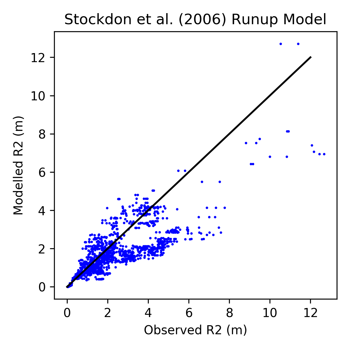
We can see there is a fair amount of scatter, especially as we get larger wave runup heights. This indicates that the model might not be working as well as we might have hoped.

Let’s also check RMSE and coefficient of determination values:

print(f"R2 Score: {r2_score(df.r2, df.sto06_r2):.2f}")
print(f"RMSE: {np.sqrt(mean_squared_error(df.r2, df.sto06_r2)):.2f} m")

Out:

R2 Score: 0.54
RMSE: 1.21 m